Which data point is driving the case for evolving dark energy?

DESI’s baryon acoustic oscillation measurements, combined with supernovae and the CMB, prefer a dark-energy equation of state that evolves with time ($w_0w_a$CDM) over a cosmological constant ($\Lambda$CDM). That preference is usually quoted as a single number for the whole dataset. But a single number hides a question worth asking:

Is the preference spread across all the data, or is it coming from one or two measurements?

Answering that requires a metric you can decompose per data point. This page introduces one — the expected log pointwise predictive density (ELPD) — and then hands you an interactive explorer to poke at the DESI DR2 result yourself.

Launch the interactive explorer →

Three different ways to score the same two models

Before ELPD, it helps to see what it is not. Given the same dataset and the same two models, here are three scores that answer three genuinely different questions:

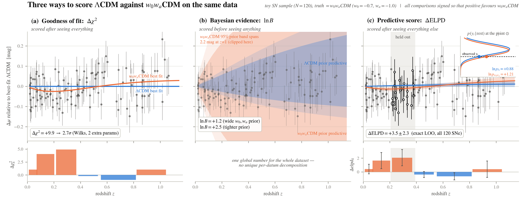
(a) Goodness of fit, $\Delta\chi^2$ — scored after seeing everything. How well does the best-fit model describe the data you already used to pick that best fit? It rewards flexibility: $w_0w_a$CDM has two extra parameters, so it can always do at least as well. You correct for that after the fact (here, Wilks’ theorem turns $\Delta\chi^2 = 9.9$ into $2.7\sigma$).

(b) Bayesian evidence, $\ln B$ — scored before seeing anything. The probability the model assigned to the data averaged over the prior. It penalises flexibility automatically, which is elegant, but the answer depends on priors you may not have strong feelings about: widening the $w_0, w_a$ prior moves $\ln B$ from $+2.5$ to $+1.2$. It also yields one global number with no unique per-datum decomposition — so it cannot tell you which point matters.

(c) Predictive score, $\Delta$ELPD — scored after seeing everything else. For each data point in turn: hide it, fit the model to the rest, and ask how much probability density the model puts on the value that was actually observed. Flexibility that only fits noise hurts you here, because the hidden point does not benefit from being fitted. Crucially, ELPD is a sum of per-point terms, so it decomposes.

That last property is the whole reason this page exists.

What ELPD actually is

For a held-out data point $y_i$, the model’s predictive density is $p(y_i \mid y_{-i})$ — the probability density the model assigns to $y_i$ after being fit to everything except $y_i$. ELPD sums the log of that over all points:

\[\mathrm{ELPD} = \sum_i \log p(y_i \mid y_{-i})\]

Each term is a genuine out-of-sample prediction, so ELPD estimates how well the model would predict new data. Comparing two models means differencing them, $\Delta\mathrm{ELPD}$, and because both the total and each per-point term subtract cleanly, you can ask “which $i$ contributes most?”

Two practical companions travel with it:

• $\hat{k}$ (Pareto $k$) — a reliability diagnostic, described below. Treat $\hat{k} > 0.7$ as “do not trust this number.”
• $p_\mathrm{loo}$ — the effective number of parameters, estimated from how much worse the model predicts held-out data than fitted data. Useful as a sanity check: for $w_0w_a$CDM vs $\Lambda$CDM you expect roughly 2 extra effective parameters, and a value far from that is a warning sign.

Why you don’t refit the model 7 times (or 1550 times)

Done literally, leave-one-out cross-validation means refitting the model once per data point. For cosmological likelihoods with MCMC, that is prohibitive.

PSIS-LOO avoids it. You fit once, then re-weight the existing posterior samples to approximate the posterior you would have obtained had point $i$ been withheld — importance sampling, where the weight for each sample is proportional to $1/p(y_i \mid \theta)$. The catch is that these weights can have very heavy tails, and a handful of samples can end up carrying all the weight, which makes the estimate unstable.

Pareto-smoothed importance sampling stabilises this by fitting a generalised Pareto distribution to the tail of the weights. The fitted shape parameter $\hat{k}$ is the diagnostic: when $\hat{k} > 0.7$, the importance-sampling estimate has no finite-variance guarantee and should not be trusted — you need an explicit refit instead. In the explorer below, withholding whole groups of tracers is informative enough to break the reweighting, and those combinations are flagged rather than silently reported.

Applying it: leave-one-tracer-out on DESI DR2

Now the cosmology. Instead of leaving out one supernova, leave out one BAO tracer — the measurement from one galaxy sample in one redshift bin (BGS, LRG1, LRG2, LRG3+ELG1, ELG2, QSO, Lyα). Every chain still contains all three probes (BAO + CMB + supernovae); what changes is which tracer’s BAO measurement is withheld and then predicted.

Watch the sign convention — it flips between the two figures on this page. The explorer writes $\Delta\mathrm{ELPD} = \Lambda\mathrm{CDM} - w_0w_a\mathrm{CDM}$, so in the explorer negative means $w_0w_a$CDM predicts that tracer better. (The toy figure above used the opposite convention.)

What to try:

1. Click a point in the top-left panel to withhold that tracer; click again to restore it. The lower panels show each model’s predictive density for the withheld tracer, on a shared axis in units of that tracer’s own error — so the measurement always sits at 0.
2. Compare the total to its uncertainty. The $\Delta$ELPD summed over the 7 BAO tracers comes with a standard error. Ask whether the aggregate preference is large compared to that spread.
3. Look for a single dominant contributor, and note that tracers pull in both directions.
4. Switch supernova compilation (Pantheon+, DES-Y5, DES-Dovekie, Union3) and see how much of the conclusion depends on that choice.
5. Use the presets to withhold all LRG bins at once — and read the $\hat{k}$ warning that appears. That warning is the methodological point of the whole exercise: the approximation tells you when it has stopped working.

The figure is dense; it works best opened in its own tab. A static PDF version is also available for citation or printing.

Where to read more

The statistical machinery here is not cosmology-specific — it comes from the Bayesian workflow literature, and the canonical references are worth reading directly:

• Vehtari, Gelman & Gabry (2017), Practical Bayesian model evaluation using leave-one-out cross-validation and WAIC, arXiv:1507.04544 — the PSIS-LOO method and the $\hat{k}$ diagnostic.
• Vehtari et al. (2024), Pareto smoothed importance sampling, arXiv:1507.02646 — the importance-sampling details.
• Gelman, Hwang & Vehtari (2014), Understanding predictive information criteria for Bayesian models, arXiv:1307.5928 — how ELPD relates to AIC, DIC, WAIC.

For the cosmology side, see my research on robust inference, and the DESI DR2 BAO cosmology results for the $w_0w_a$CDM preference itself.

Questions, or spotted something wrong? Get in touch.